Purpose
The purposes of this exercise to look into different features to observe their relationship, and plot a multiple linear regression based on several features of individual such as age, body mass index (bmi), gender etc to be used for predicting future medical expenses of individuals that help medical insurance to make decision on charging the premium.
Predicting Insurance Premiums
Our simple dataset contains a few attributes for each person such as Age, Sex, BMI, Children, Smoker, Region and their charges
Aim
To use this info to predict charges for new customers
Machine Learning Algorithms used in the case study
This is a free case study on data science, where we are going to show how to use different machine learning algorithms like Multiple Linear Regression, Support Vector Machine Regression, Random Forest regression and predict the insurance premium. It's a total step by step tutorial to learn how to use a machine learning algorithm using Python to help a business to take decision.
We are going to import the data into Python
import numpy as np
import pandas as pd
import os
import matplotlib.pyplot as plt
pd.options.mode.chained_assignment = None  # removes warning messages


os.chdir("C:\\Users\\ASUS")
insurance = pd.read_csv("insurance.csv")

# Preview our data
insurance.head()
| age | sex | bmi | children | smoker | region | charges | |
|---|---|---|---|---|---|---|---|
| 0 | 19 | female | 27.900 | 0 | yes | southwest | 16884.92400 |
| 1 | 18 | male | 33.770 | 1 | no | southeast | 1725.55230 |
| 2 | 28 | male | 33.000 | 3 | no | southeast | 4449.46200 |
| 3 | 33 | male | 22.705 | 0 | no | northwest | 21984.47061 |
| 4 | 32 | male | 28.880 | 0 | no | northwest | 3866.85520 |
# Showing the properties of different variables
insurance.info()
<class 'pandas.core.frame.DataFrame'>
RangeIndex: 1338 entries, 0 to 1337
Data columns (total 7 columns):
 #   Column    Non-Null Count  Dtype
---  ------    --------------  -----
 0   age       1338 non-null   int64
 1   sex       1338 non-null   object
 2   bmi       1338 non-null   float64
 3   children  1338 non-null   int64
 4   smoker    1338 non-null   object
 5   region    1338 non-null   object
 6   charges   1338 non-null   float64
dtypes: float64(2), int64(2), object(3)
memory usage: 73.3+ KB
insurance.isnull().sum()
age         0
sex         0
bmi         0
children    0
smoker      0
region      0
charges     0
dtype: int64
insurance.corr()
| age | bmi | children | charges | |
|---|---|---|---|---|
| age | 1.000000 | 0.109272 | 0.042469 | 0.299008 |
| bmi | 0.109272 | 1.000000 | 0.012759 | 0.198341 |
| children | 0.042469 | 0.012759 | 1.000000 | 0.067998 |
| charges | 0.299008 | 0.198341 | 0.067998 | 1.000000 |
Univariate analysis
fig, axes = plt.subplots(nrows=2, ncols=2, figsize=(12, 10))
insurance.plot(kind="hist", y="age", bins=70, color="b", ax=axes[0][0])
insurance.plot(kind="hist", y="bmi", bins=100, color="r", ax=axes[0][1])
insurance.plot(kind="hist", y="children", bins=6, color="g", ax=axes[1][0])
insurance.plot(kind="hist", y="charges", bins=100, color="orange", ax=axes[1][1])
plt.show()

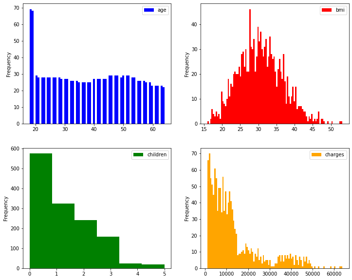
Observations: We can see that all these variables are having variations. BMI seems to be almost a normally distributed.
Bivariate analysis
import seaborn as sns  # Imorting Seaborn library
#pal = ["#FA5858", "#58D3F7"]
sns.scatterplot(x="bmi", y="charges", data=insurance, palette=pal, hue='smoker')
<AxesSubplot:xlabel='bmi', ylabel='charges'>

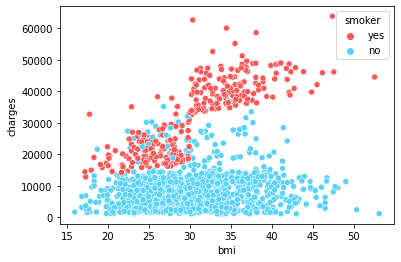
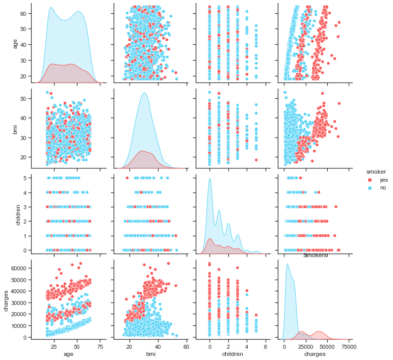
Observations: It's pretty clear that smokers are paying a higher premium than non-smokers. BMI doesn't seem to impacting the charges much.
import seaborn as sns

sns.set(style="ticks")
pal = ["#FA5858", "#58D3F7"]

sns.pairplot(insurance, hue="smoker", palette=pal)
plt.title("Smokers")
Text(0.5, 1.0, 'Smokers')

Preparing Data for Machine Learning Algorithms
insurance.head()
| age | sex | bmi | children | smoker | region | charges | |
|---|---|---|---|---|---|---|---|
| 0 | 19 | female | 27.900 | 0 | yes | southwest | 16884.92400 |
| 1 | 18 | male | 33.770 | 1 | no | southeast | 1725.55230 |
| 2 | 28 | male | 33.000 | 3 | no | southeast | 4449.46200 |
| 3 | 33 | male | 22.705 | 0 | no | northwest | 21984.47061 |
| 4 | 32 | male | 28.880 | 0 | no | northwest | 3866.85520 |
insurance=pd.get_dummies(data=insurance,columns=['sex', 'smoker',"region"],drop_first=True)
All the dummy variables have been properly created
insurance.head(3)
| age | bmi | children | charges | sex_male | smoker_yes | region_northwest | region_southeast | region_southwest | |
|---|---|---|---|---|---|---|---|---|---|
| 0 | 19 | 27.90 | 0 | 16884.9240 | 0 | 1 | 0 | 0 | 1 |
| 1 | 18 | 33.77 | 1 | 1725.5523 | 1 | 0 | 0 | 1 | 0 |
| 2 | 28 | 33.00 | 3 | 4449.4620 | 1 | 0 | 0 | 1 | 0 |
#segregate data into dependent and independent variables

X = insurance.drop("charges", axis = 1)#independent variables
y = insurance["charges"]#dependent variable
Now we will split the data into training (80% of the data) and rest 30% - named test, will be kept aside for later use.
# Splitting it into training and testing (70% train & 30% test)
from sklearn.model_selection import train_test_split
X_train, X_test, y_train, y_test = train_test_split(X, y, test_size = 0.3, random_state = 42)
We are concatenating the train and test so that we can easily use it for Linear regression. Later, we will use it (without concatenating) for SVM and Random Forest algorithms.
# Concatenating the training data to create a single dataset
df = pd.concat([y_train,X_train],axis=1)
df.head()
| charges | age | bmi | children | sex_male | smoker_yes | region_northwest | region_southeast | region_southwest | |
|---|---|---|---|---|---|---|---|---|---|
| 332 | 13429.03540 | 61 | 31.160 | 0 | 0 | 0 | 1 | 0 | 0 |
| 355 | 24603.04837 | 46 | 27.600 | 0 | 1 | 0 | 0 | 0 | 1 |
| 138 | 27322.73386 | 54 | 31.900 | 3 | 0 | 0 | 0 | 1 | 0 |
| 381 | 42303.69215 | 55 | 30.685 | 0 | 1 | 1 | 0 | 0 | 0 |
| 292 | 42112.23560 | 25 | 45.540 | 2 | 1 | 1 | 0 | 1 | 0 |
import statsmodels.formula.api as sm
rock=sm.ols(formula=
"""charges ~ age+ bmi + children + sex_male + smoker_yes +
region_northwest + region_southeast + region_southwest""",
data=df).fit()
rock.summary()# shows total summary
| Dep. Variable: | charges | R-squared: | 0.742 |
|---|---|---|---|
| Model: | OLS | Adj. R-squared: | 0.740 |
| Method: | Least Squares | F-statistic: | 333.9 |
| Date: | Wed, 22 Jun 2022 | Prob (F-statistic): | 6.51e-267 |
| Time: | 21:11:58 | Log-Likelihood: | -9492.8 |
| No. Observations: | 936 | AIC: | 1.900e+04 |
| Df Residuals: | 927 | BIC: | 1.905e+04 |
| Df Model: | 8 | ||
| Covariance Type: | nonrobust |
| coef | std err | t | P>|t| | [0.025 | 0.975] | |
|---|---|---|---|---|---|---|
| Intercept | -1.237e+04 | 1210.540 | -10.222 | 0.000 | -1.47e+04 | -9998.247 |
| age | 261.2969 | 14.435 | 18.102 | 0.000 | 232.968 | 289.626 |
| bmi | 348.9069 | 35.285 | 9.888 | 0.000 | 279.659 | 418.154 |
| children | 424.1191 | 166.972 | 2.540 | 0.011 | 96.432 | 751.806 |
| sex_male | 104.8118 | 404.887 | 0.259 | 0.796 | -689.790 | 899.413 |
| smoker_yes | 2.363e+04 | 498.610 | 47.388 | 0.000 | 2.26e+04 | 2.46e+04 |
| region_northwest | -486.9346 | 570.048 | -0.854 | 0.393 | -1605.668 | 631.799 |
| region_southeast | -970.9688 | 579.867 | -1.674 | 0.094 | -2108.973 | 167.036 |
| region_southwest | -926.3229 | 578.431 | -1.601 | 0.110 | -2061.509 | 208.863 |
| Omnibus: | 224.792 | Durbin-Watson: | 2.075 |
|---|---|---|---|
| Prob(Omnibus): | 0.000 | Jarque-Bera (JB): | 543.466 |
| Skew: | 1.270 | Prob(JB): | 9.73e-119 |
| Kurtosis: | 5.735 | Cond. No. | 311. |
Notes:
[1] Standard Errors assume that the covariance matrix of the errors is correctly specified.
Remove insignificant variables (p value more than 0.05) and lowest absolute t value; one variable at a time.
# Remove first sex_male followed by region_northwest
import statsmodels.formula.api as sm
rock=sm.ols(formula=
"""charges ~ age+ bmi + children  + smoker_yes +
 region_southeast + region_southwest""",
data=insurance).fit()
rock.summary()# shows total summary
| Dep. Variable: | charges | R-squared: | 0.751 |
|---|---|---|---|
| Model: | OLS | Adj. R-squared: | 0.750 |
| Method: | Least Squares | F-statistic: | 668.3 |
| Date: | Wed, 22 Jun 2022 | Prob (F-statistic): | 0.00 |
| Time: | 21:12:09 | Log-Likelihood: | -13548. |
| No. Observations: | 1338 | AIC: | 2.711e+04 |
| Df Residuals: | 1331 | BIC: | 2.715e+04 |
| Df Model: | 6 | ||
| Covariance Type: | nonrobust |
| coef | std err | t | P>|t| | [0.025 | 0.975] | |
|---|---|---|---|---|---|---|
| Intercept | -1.217e+04 | 949.538 | -12.812 | 0.000 | -1.4e+04 | -1.03e+04 |
| age | 257.0064 | 11.889 | 21.617 | 0.000 | 233.683 | 280.330 |
| bmi | 338.6413 | 28.554 | 11.860 | 0.000 | 282.625 | 394.657 |
| children | 471.5441 | 137.656 | 3.426 | 0.001 | 201.498 | 741.590 |
| smoker_yes | 2.384e+04 | 411.659 | 57.921 | 0.000 | 2.3e+04 | 2.47e+04 |
| region_southeast | -858.4696 | 415.206 | -2.068 | 0.039 | -1672.998 | -43.941 |
| region_southwest | -782.7452 | 413.756 | -1.892 | 0.059 | -1594.430 | 28.940 |
| Omnibus: | 300.125 | Durbin-Watson: | 2.092 |
|---|---|---|---|
| Prob(Omnibus): | 0.000 | Jarque-Bera (JB): | 716.587 |
| Skew: | 1.211 | Prob(JB): | 2.48e-156 |
| Kurtosis: | 5.643 | Cond. No. | 295. |
Notes:
[1] Standard Errors assume that the covariance matrix of the errors is correctly specified.
Anova (Prob (F-statistic)) is less than 0.05, which ideally should be the case
p value of region_southwest (0.059) is slightly more than 0.05, but we can safely ignore it and let the variable be in the model
R-squared (0.751 ~ 75.1%) and Adj. R-squared (0.750 ~ 75%) are pretty high (closer to 1 better the model) and very close to each other. It shows that our independent variables can explain about 75% of the variance of dependent variable (charges)
var = pd.DataFrame(round(rock.pvalues,3))# shows p value
#var["coeff"] = rock.params#coefficients
from statsmodels.stats.outliers_influence import variance_inflation_factor
variables = rock.model.exog #.if I had saved data as rock
# this it would have looked like rock.model.exog
vif = [variance_inflation_factor(variables, i) for i in range(variables.shape[1])]
vif
var["vif"] = vif
var
| 0 | vif | |
|---|---|---|
| Intercept | 0.000 | 32.859280 |
| age | 0.000 | 1.016174 |
| bmi | 0.000 | 1.104196 |
| children | 0.001 | 1.002831 |
| smoker_yes | 0.000 | 1.005747 |
| region_southeast | 0.039 | 1.244250 |
| region_southwest | 0.059 | 1.147367 |
Predicting the price for the test data
# Creating a single dataset with the testing data
df1 = pd.concat([y_test,X_test],axis=1)
#predict the test data with the model
df1["pred"] = rock.predict(X_test)
df1.head()
| charges | age | bmi | children | sex_male | smoker_yes | region_northwest | region_southeast | region_southwest | pred | |
|---|---|---|---|---|---|---|---|---|---|---|
| 764 | 9095.06825 | 45 | 25.175 | 2 | 0 | 0 | 0 | 0 | 0 | 8868.289033 |
| 887 | 5272.17580 | 36 | 30.020 | 0 | 0 | 0 | 1 | 0 | 0 | 7252.860495 |
| 890 | 29330.98315 | 64 | 26.885 | 0 | 0 | 1 | 1 | 0 | 0 | 37231.273781 |
| 1293 | 9301.89355 | 46 | 25.745 | 3 | 1 | 0 | 1 | 0 | 0 | 9789.865128 |
| 259 | 33750.29180 | 19 | 31.920 | 0 | 1 | 1 | 1 | 0 | 0 | 27371.045323 |
Calculate the accuracy of the model
from sklearn.metrics import mean_absolute_percentage_error
mean_absolute_percentage_error(df1["charges"],df1["pred"])*100
42.1614163772496
MAPE of 42.14% means the predicted values are 42.14% deviated from the actual values. We can assume this model has an accuracy of 100%- 42.14% = 57.86% of accuracy. This is rather poor accuracy.
Now we will be using Support Vector Machine (SVM)
We will do the feature scaling first
# Feature Scaling
from sklearn.preprocessing import StandardScaler
sc = StandardScaler()
X_train = sc.fit_transform(X_train)
X_test = sc.transform(X_test)
from sklearn.svm import SVR
svr = SVR(kernel = 'rbf')
svr.fit(X_train, y_train)
SVR()
Predict the charges
# Predict the model
y_pred = svr.predict(X_test)
from sklearn.metrics import mean_absolute_percentage_error
mean_absolute_percentage_error(y_test,y_pred)*100
103.25108812337018
Method 2 - manually by creating a data frame
d = pd.DataFrame()
d["test_y"] = y_test
d["y_pred"] = y_pred

#Mape with formula
d["mp"] = abs((d["test_y"]- d["y_pred"])/d["test_y"])
(d.mp.mean())*100#mape
103.25108812337018
We are getting a mape of 103% (absolutely not acceptable) which means Support Vector Regression (SVR) is not suitable for this data.
We will try with the hyper parameter tuning and try to improve the mape
parameters={"kernel":['linear', 'poly', 'rbf', 'sigmoid'],
'gamma': ['scale', 'auto'] }
from sklearn.model_selection import GridSearchCV
grid_search = GridSearchCV(estimator = svr,
param_grid = parameters, n_jobs = -1)#n_jobs = -1 will apply all CPUs

grid_search.fit(X_train, y_train)

y_pred = grid_search.predict(X_test)
optimal hyper-parameters
grid_search.best_params_
{'gamma': 'scale', 'kernel': 'linear'}
Calculate MAPE after hyper-parameters tuning
from sklearn.metrics import mean_absolute_percentage_error
mean_absolute_percentage_error(y_test,y_pred)*100
92.1504136167104
We can see that the mape has improved but still it's very high and not acceptable.
Now we will be using Random Forest algorithm
from sklearn.ensemble import RandomForestRegressor
rf = RandomForestRegressor(n_estimators = 1000, random_state = 42)
rf.fit(X_train, y_train)
RandomForestRegressor(n_estimators=1000, random_state=42)
Predict the charges
# Predict the model
y_pred = rf.predict(X_test)
from sklearn.metrics import mean_absolute_percentage_error
mean_absolute_percentage_error(y_test,y_pred)*100
33.09156255231602
Method 2 - manually by creating a data frame
d = pd.DataFrame()
d["test_y"] = y_test
d["y_pred"] = y_pred

#Mape with formula
d["mp"] = abs((d["test_y"]- d["y_pred"])/d["test_y"])
(d.mp.mean())*100#mape
33.09156255231602
We are getting a mape of 33%, it seems that Random Forest has performed the best among all the 3 algorithms
Now let's try again with the hyper-parameters if MAPE can be further improved
#Set the parameters
parameters={"max_depth":[5,10,15],
'min_samples_leaf': [3, 4, 5] }
#Set the grid search
from sklearn.model_selection import GridSearchCV
grid_search = GridSearchCV(estimator = rf,
param_grid = parameters, n_jobs = -1)#n_jobs = -1 will apply all CPUs
# Execute the grid search
grid_search.fit(X_train, y_train)
GridSearchCV(estimator=RandomForestRegressor(n_estimators=1000,
                                             random_state=42),
             n_jobs=-1,
             param_grid={'max_depth': [5, 10, 15],
                         'min_samples_leaf': [3, 4, 5]})
Predict and Calculate MAPE
y_pred = grid_search.predict(X_test)
from sklearn.metrics import mean_absolute_percentage_error
mean_absolute_percentage_error(y_test,y_pred)*100
29.846981277483508