PROBLEM STATEMENT : T Shirt size prediction using the Machine Learning algorithm K Nearest Neighbor (KNN). We will use Python to build this model.
Today we're going to discuss a famous classification algorithm, which is called K Nearest Neighbors or KNN and all right, the name might look a little bit intimidating, but trust me, it's actually very, very simple algorithm, very intuitive. And in this blog, what I'm going to do is we are going to walk you through kind of a practical example to take a look at the nearest neighbor.
So this neighbor algorithm is a classification algorithm, so we're expecting the output to be categorical or to be binary. So either, let's say we want to predict the t shirt size, small, medium or large. Let's say, you want to predict if someone is healthy or sick, going to pass or fail and so on.
That's kind of the idea or the expected output when we apply the k nearest neighbor and it works by finding the most similar data points in the training data and attempt to make an educated guess based on their classification.
I know it might look, you know, what are you talking about? Let's take a look at an example. And that will would be very clear afterwards.
You own an online clothing business and you would like to develop a new app (or in-store) feature in which customers would enter their own height and weight and the system would predict what T-shirt size should they wear. Features are height and weight and output is either L (Large) or S (Small).
OK, so the customer, we're going to walk in, let's say, in the store and what are we going to do? We're going to ask the customers to provide us with their weight in kilograms, which is the first feature and the second feature, which is going to be height in centimeters. Right. So these are kind of the inputs to the algorithm. And the algorithm should predict whether we wanted to give him or provide the customer with either size large. Let's say in-store feature where the customer we're going to walk in, provided that with the two features, their weight in kilograms and their height in centimeters. And what we're going to predict for them and get them, you know what we're going to give you either size, small or size large based on it.
Import the packages
import pandas as pd
import numpy as np
import matplotlib.pyplot as plt
import seaborn as sns
%matplotlib inline
import os
We will import the data
os.chdir("D:\\Python")
Tshirt = pd.read_csv("Tshirt_Sizing_Dataset.csv")
Tshirt.head(10)
| Height (in cms) | Weight (in kgs) | T Shirt Size | |
|---|---|---|---|
| 0 | 158 | 58 | S |
| 1 | 158 | 59 | S |
| 2 | 158 | 63 | S |
| 3 | 160 | 59 | S |
| 4 | 160 | 60 | S |
| 5 | 163 | 60 | S |
| 6 | 163 | 61 | S |
| 7 | 160 | 64 | L |
| 8 | 163 | 64 | L |
| 9 | 165 | 61 | L |
In this data Height and Weight are given; these are my indementdent variables. T shirt size is my dependent variable. Using the Height and Weight we will predict the T shirt size.
Checking for missing values
# number of missing values by variables
Tshirt.isnull().sum()
Height (in cms)    0
Weight (in kgs)    0
T Shirt Size       0
dtype: int64
Observation: There are no missing values in the data
X = Tshirt.drop("T Shirt Size",axis=1)
y = Tshirt.loc[:, "T Shirt Size"]
We need to change the t shirt size to numeric. Hence we will be using one hot lebel encoder to change it.
from sklearn.preprocessing import LabelEncoder
labelencoder_y = LabelEncoder()
y = labelencoder_y.fit_transform(y)
Now we will split the data into training (75% of the data) and rest 25% - named test, will be kept aside for later use.
from sklearn.model_selection import train_test_split
X_train, X_test, y_train, y_test = train_test_split(X, y, test_size=0.25)
# Feature Scaling
# from sklearn.preprocessing import StandardScaler
# sc = StandardScaler()
# X_train = sc.fit_transform(X_train)
# X_test = sc.transform(X_test)
STEP#3: MODEL TRAINING
# Fitting K-NN to the Training set
from sklearn.neighbors import KNeighborsClassifier
classifier = KNeighborsClassifier(n_neighbors = 5, metric = 'minkowski', p = 2)
classifier.fit(X_train, y_train)
KNeighborsClassifier(algorithm='auto', leaf_size=30, metric='minkowski',
           metric_params=None, n_jobs=1, n_neighbors=5, p=2,
           weights='uniform')
STEP#4: MODEL TESTING
# Predicting the Test set results
y_pred = classifier.predict(X_test)
y_pred
array([0, 1, 0, 1, 0], dtype=int64)
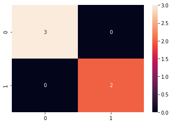
# Making the Confusion Matrix
from sklearn.metrics import confusion_matrix
cm = confusion_matrix(y_test, y_pred)
sns.heatmap(cm, annot=True, fmt="d")
<matplotlib.axes._subplots.AxesSubplot at 0x20e1ae42a90>
STEP#5: TESTING RESULTS VISUALIZATION
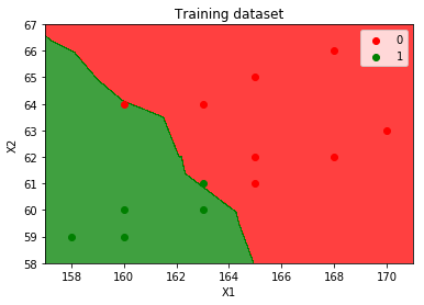
VISUALIZE TRAINING SET RESULTS
# Visualising the Training set results
from matplotlib.colors import ListedColormap
X_grid, y_grid = X_train, y_train
X1, X2 = np.meshgrid(np.arange(start = X_grid[:, 0].min() - 1, stop = X_grid[:, 0].max() + 1, step = 0.01),
                     np.arange(start = X_grid[:, 1].min() - 1, stop = X_grid[:, 1].max() + 1, step = 0.01))
plt.contourf(X1, X2, classifier.predict(np.array([X1.ravel(), X2.ravel()]).T).reshape(X1.shape), alpha = 0.75, cmap = ListedColormap(('red', 'green')))
plt.xlim(X1.min(), X1.max())
plt.ylim(X2.min(), X2.max())
for i, j in enumerate(np.unique(y_grid)):
    plt.scatter(X_grid[y_grid == j, 0], X_grid[y_grid == j, 1],
                c = ListedColormap(('red', 'green'))(i), label = j)

plt.title('Training dataset')
plt.xlabel('X1')
plt.ylabel('X2')
plt.legend()
plt.show()
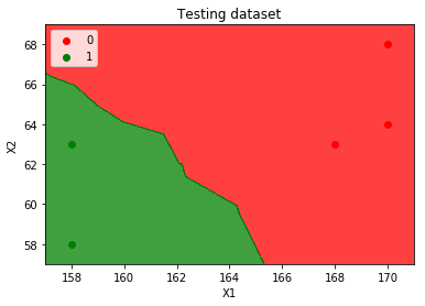
VISUALIZE TEST SET RESULTS
# Visualising the Training set results
from matplotlib.colors import ListedColormap
X_grid, y_grid = X_test, y_test
X1, X2 = np.meshgrid(np.arange(start = X_grid[:, 0].min() - 1, stop = X_grid[:, 0].max() + 1, step = 0.01),
                     np.arange(start = X_grid[:, 1].min() - 1, stop = X_grid[:, 1].max() + 1, step = 0.01))
plt.contourf(X1, X2, classifier.predict(np.array([X1.ravel(), X2.ravel()]).T).reshape(X1.shape), alpha = 0.75, cmap = ListedColormap(('red', 'green')))
plt.xlim(X1.min(), X1.max())
plt.ylim(X2.min(), X2.max())
for i, j in enumerate(np.unique(y_grid)):
    plt.scatter(X_grid[y_grid == j, 0], X_grid[y_grid == j, 1], c = ListedColormap(('red', 'green'))(i), label = j)

plt.title('Testing dataset')
plt.xlabel('X1')
plt.ylabel('X2')
plt.legend()
plt.show()